Vectors and scalars
1.3.1 Distinguish between vector and scalar quantities, and give examples of each.
When expressing a quantity we give it a number and a unit (for example, 12 kg), this expresses the magnitude of the quantity. Some quantities also have direction, a quantity that has both a magnitude and direction is called a vector. On the other hand, a quantity that has only a magnitude is called a scalar quantity. Vectors are represented in print as bold and italicised characters (for example F). Below is a table listing some vector and scalar quantities:
| Scalars | Vectors |
| Speed | Velocity |
| Temperature | Acceleration |
| Distance | Displacement |
| Area | Force |
| Entropy | Momentum |
| Volume | Drag |
Table 1.3.1 - Vector and scalar quantites
Note that some quantities appear to be the same, such as velocity and speed, both representing distance over time, the difference is that velocity has a direction whilst speed does not.
1.3.2 Determine the sum or difference of two vectors by a graphical method.
The difference of two vectors
When adding vectors, we need to take both the magnitude and direction into account. Often, we will have situations where two vectors have opposite directions, in this case, we simply subtract the smallest magnitude from the largest one. This is demonstrated in figure 1.3.1 below:
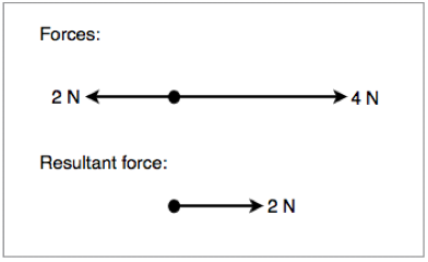
Figure 1.3.1 - Resultant force of two opposing vectors
The sum of two vectors
Sometimes we will have situations where two forces are acting in the same direction. In the situations we simply add together the magnitudes of both vectors. This is demonstrated in figure 1.3.2 below:
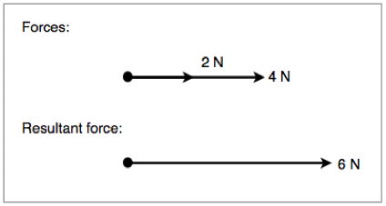
Figure 1.3.2 - Resultant force of two concurrent vectors
Adjacent vectors
In certain situations, we will need to work out the angle between two adjacent vectors. In order to do this graphically we draw a scale diagram with the tail of one vector at the head of the other, we then draw a line connecting the other head and tail. To get the magnitude of the new vector, we simply measure it. This is demonstrated in the diagram below:
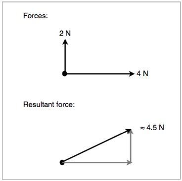
Figure 1.3.3 - Graphical method of solving adjacent vectors
Alternatively, we can use trigonometry for a faster and more accurate result. This is demonstrated in figure 1.3.4 below:
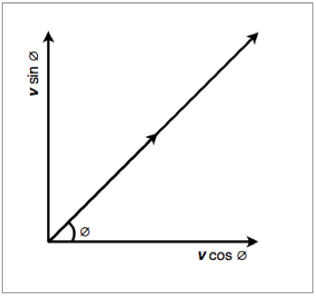
Figure 1.3.4 - Trigonometric method of solving adjacent vectors
Scalar multiplication
We can also multiply (and divide) vectors by scalars. When doing so we follow a set of rules:
- Multiplying by 1 does not change a vector 1 v = v
- Multiplying by 0 gives the null vector 0 v = 0
- Multiplying by -1 gives the additive inverse -1 v = -v
- Left distributivity: (c + d)v = cv + dv
- Right distributivity: c(v + w) = cv + cw
- Associativity: (cd)v = c(dv)
Scalar multiplication is demonstrated in figure 1.3.5 below:
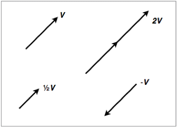
Figure 1.3.5 - Scalar multiplication and division of vectors
1.3.3 Resolve vectors into perpendicular components along chosen axes.
When working with adjacent vectors that do not form a 90° angle, it is often useful to brake certain vectors into component vectors so that they are concurrent with the other vectors. To do this, we draw two vectors, one horizontal and the other vertical to our plane of reference. We then use trigonometry to work out the magnitude of each new vector and figure out the resulting force. This is shown in figure 1.3.6 and 1.3.7:
Figure 1.3.6 shows a diagram of the forces acting on a block being pushed along a smooth surface:
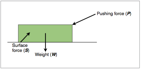
Figure 1.3.6 - Forces acting on a block
Figure 1.3.7 shows the same diagram but with the surface and pushing forces broken down into their components:
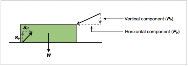
Figure 1.3.7 - Forces acting on a block broken into their components
Sometimes the plane of reference will not be parallel to the page, such and example is shown in figure 1.3.8 below:

Figure 1.3.8 - Component forces of a block on a slope